
The journey began with a spark of inspiration from Twitter. When I came across Dylan Drummey’s post about bat keypoint tracking with MLB video, I immediately recognized its potential application at Driveline Baseball. That same day, I dove headfirst into the project by beginning to annotate 1,000 side-view hitting images.
This article was written by Clayton Thompson and Adam Bloebaum in the Driveline R&D department.
Understanding Annotation and Model Training
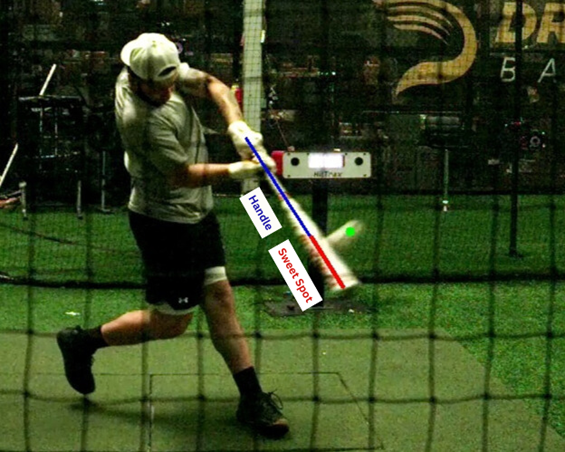
Annotation is a crucial first step in training computer vision models. Think of it as teaching a child to recognize objects – you first need to show them many examples while pointing out what they’re looking at. In our case, we were teaching our model to recognize two specific points on a baseball bat: the cap (end) and the knob (handle). This process involved manually marking these points on thousands of images, creating a dataset of precise pixel coordinates for each keypoint.
This annotation process is fundamental to pose estimation models, which differ from traditional object detection models. While object detection tells you where an object is in an image (like finding a bat), pose estimation goes further by identifying specific points on that object (like pinpointing exactly where the cap and knob are). By providing thousands of examples of correctly labeled keypoints, we’re essentially creating a training manual for the model to learn the visual patterns that indicate these specific locations.
Model Architecture
While we had previous experience using YOLOv8 for computer vision tasks at Driveline Baseball, this project required a different approach. We needed a custom pose estimation model specifically designed to track bat keypoints. This was our first venture into training a custom pose model, and it came with its own set of challenges.
The initial results were promising – our model could track the bat’s movement relatively well. However, our ultimate goal was more ambitious: we wanted to estimate bat speed from simple side-view video. This meant we needed to build a comprehensive dataset pairing side-view video swings with our marker-based motion capture data to provide ground truth velocities for training.
Data Collection Pipeline
Our first major undertaking was setting up a robust data collection system. We repurposed a 2014 Edgertronic SC1 camera, synchronizing it with our lab setup to automatically trigger with every swing in the mocap lab. The real challenge wasn’t just collecting the data – it was ensuring perfect pairing between our mocap data and side-view videos. We spent nearly a month developing sophisticated pipelines to automatically match and verify this data each night.
Processing and Point of Contact Detection
With our data collection system in place, we faced our next challenge: identifying the key frames in each swing. While we had the pixel positions of the cap and knob, we needed a reliable way to identify the point of contact. Our initial approach of using cap velocity to detect the start of the swing proved too inconsistent, so we shifted our focus to finding the point of contact.
This led us to develop another model, this time for ball detection. We manually annotated approximately 10,000 images, but we worked smarter by implementing semi-automatic annotation. Our existing model could predict ball locations, which we used to assist in drawing detection bounding boxes. This significantly accelerated our annotation process while maintaining accuracy.
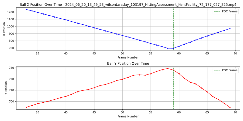
Determining the exact point of contact required careful consideration. In a right-side view video, the ball typically moves right to left through the frame. We initially tried to identify point of contact by detecting the first frame where the ball changed direction, but this approach came with significant limitations.
Our initial method required the ball to first appear in the right third of the frame and show movement in the subsequent frame. This strict requirement, combined with our model’s tendency to generate false positives, created reliability issues. We needed a robust method to filter out outlier detections while maintaining the ability to track the ball’s complete trajectory.
The handedness of the batter introduced additional complexity. Since our algorithm expected right-to-left ball movement, we had to flip all left-handed hitter videos to appear right-handed. This wasn’t just about ball tracking – we wanted our positional keypoints for left-handed swings to mirror and match our right-handed data for consistency in our analysis. For example, all of Adam’s test swings had to be flipped to maintain this standardization.
Our solution evolved to use both bat and ball positions, finding the frame where the ball was closest to the bat’s sweet spot (defined as 1/3 of the distance from the cap to the knob). We ultimately chose to use the frame just before actual contact as our reference point.
The Scaling Factor Challenge
One of our most significant challenges came from an unexpected source: perspective. Different hitters naturally stand at varying distances from the camera, which created a fundamental problem in our 2D to 3D coordinate conversion. Our initial attempt to solve this through position normalization proved to be a critical mistake, one that had far-reaching implications for our bat speed predictions.
The normalization approach essentially forced all swings into the same positional constraints, regardless of their actual spatial relationships. This was like trying to measure the height of buildings by making all their photographs the same size – you lose the crucial information about their true scale. But the problem went deeper than just spatial relationships. By normalizing the positions, we were inadvertently altering the fundamental physics of each swing.
# Get the overall range for x and y coordinates
x_min = min(df['x1'].min(), df['x2'].min())
y_min = min(df['y1'].min(), df['y2'].min())
x_max = min(df['x1'].max(), df['x2'].max())
y_max = min(df['y1'].max(), df['y2'].max())

# Normalize all coordinates using the same range
df['x1_norm'] = (df['x1'] - x_min) / (x_max - x_min)
df['x1_norm'] = (df['x1'] - x_min) / (x_max - x_min)
df['y1_norm'] = (df['y1'] - y_min) / (y_max - y_min)
df['y2_norm'] = (df['y2'] - y_min) / (y_max - y_min)
In baseball, longer swings provide more time for acceleration, allowing the bat to potentially achieve higher speeds. When we normalized our position data, we were effectively compressing or expanding these swing paths artificially. A long, powerful swing taken from far away might be compressed to look like a shorter swing, while a compact swing taken close to the camera might be stretched out. This normalization was essentially erasing the natural relationship between swing path length and potential bat speed, making our velocity predictions unreliable. As a result, our model was quite poor.
We first attempted to solve this using monocular depth modeling – a technique that tries to estimate depth from a single camera view. While the approach showed promise in extracting depth information from our 2D videos, it proved too computationally intensive and inconsistent for real-time analysis.
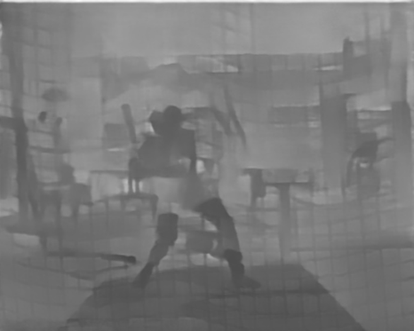
The arbitrary nature of depth predictions from a single viewpoint made it difficult to establish reliable measurements across different swings and batting stances. Depth maps were generated by a neural network for each frame which was used to get keypoint depth.
The breakthrough came when we realized we could use the bat itself as a reference object. Since we know the actual length of a bat, we could calculate a scaling factor based on its apparent size in the video:
scaling_factor = actual_bat_length / max_apparent_bat_length
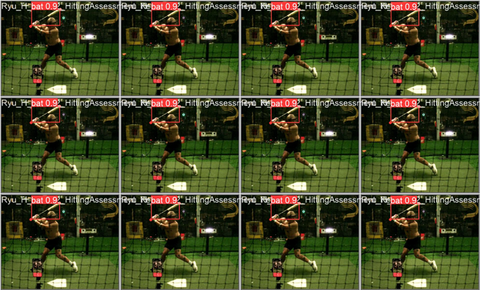
This elegant solution provided a proxy for depth, as a bat appears smaller when further from the camera and larger when closer. Initially, we considered using the apparent bat length at point of contact to determine our scaling factor. Let’s look at some examples that illustrate both the promise and limitations of this approach:
Looking at two left-handed hitters, we see similar apparent bat lengths around point of contact, suggesting this could be a reliable depth proxy.
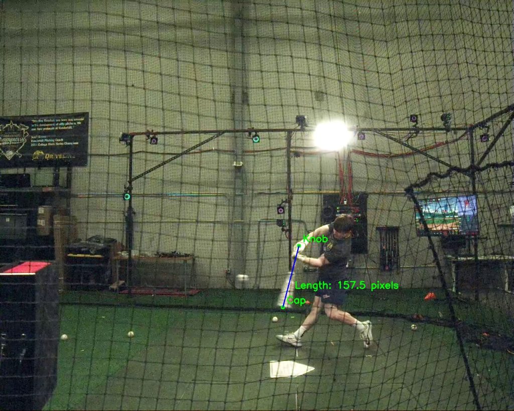
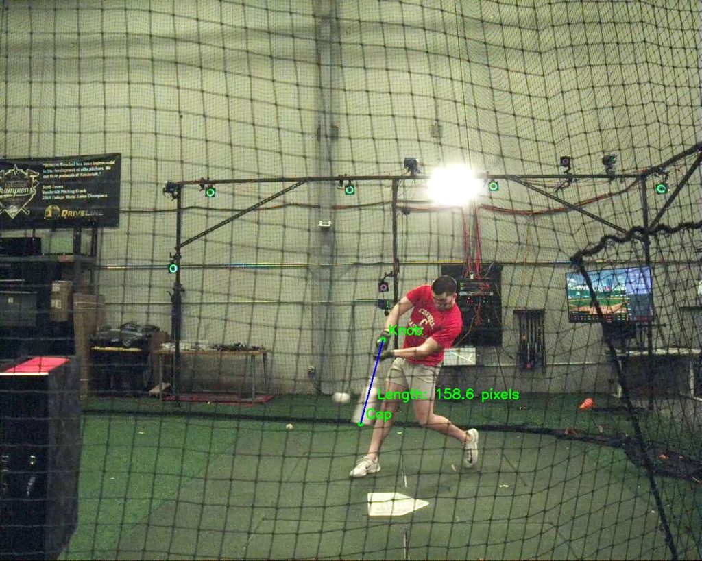
When examining right-handed hitters, we found consistently larger apparent bat lengths – exactly what we’d expect since they stand closer to the camera. This validated our basic premise: apparent bat length could indeed indicate relative depth. However, we also observed nearly 20-pixel differences between right-handed swings at similar distances.
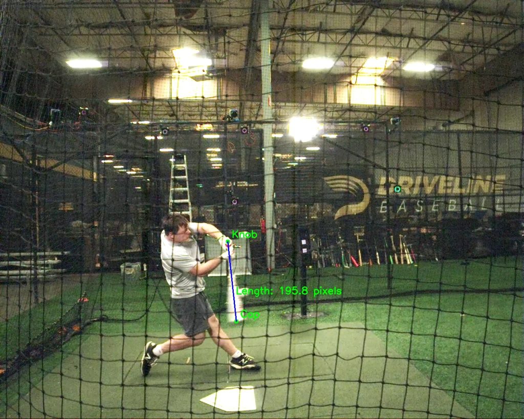
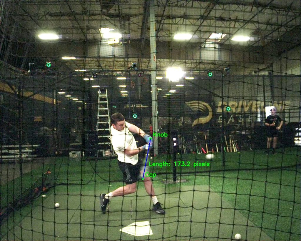
While apparent bat length can indicate depth, it’s significantly affected by vertical bat angle. This led us to modify our approach. Instead of using the bat length at point of contact, we decided to use the maximum apparent bat length throughout the entire swing.
# Euclidian Distance to get bat length for each frame
np_bat_length = np.sqrt((df['x2'] - df['x1'])**2 + (df['y2'] - df['y1'])**2)

# Getting maximum appearing bat length
max_appearing_bat_length = np_bat_length.max()

# Calculation of the scaling factor
scaliing_factor = bat_length / max_appearing_bat_length
This proved more robust because it reduced the impact of vertical bat angle variations. We don’t need to know the exact distance from the camera – we just need a reliable way to tell if one hitter is generally closer or further away than another.
With this refined approach, we applied the scaling factor to our positional data:
x_scaled = pos_x * scaling_factor
This method dramatically improved our model’s accuracy by preserving both true spatial relationships and natural swing dynamics. The beauty of this solution lies in its simplicity – we’re using the bat itself to tell us approximately how far away the hitter is standing.
Data Smoothing and Signal Processing
The Butterworth filter is particularly favored in biomechanics because of its “maximally flat” frequency response – meaning it minimizes distortion of the true signal within its passband. This characteristic makes it ideal for human movement analysis, where maintaining the integrity of the movement pattern while removing sensor noise is crucial. In traditional biomechanics applications like gait analysis or pitching mechanics, these filters effectively separate the relatively low-frequency human movement from high-frequency noise.
However, bat swing analysis presented a unique challenge that made traditional biomechanics filtering approaches less suitable. Bat speed can change extremely rapidly during a swing, with the fastest acceleration occurring just before contact. These rapid changes in velocity create high-frequency components in our signal that are actually meaningful data, not noise.
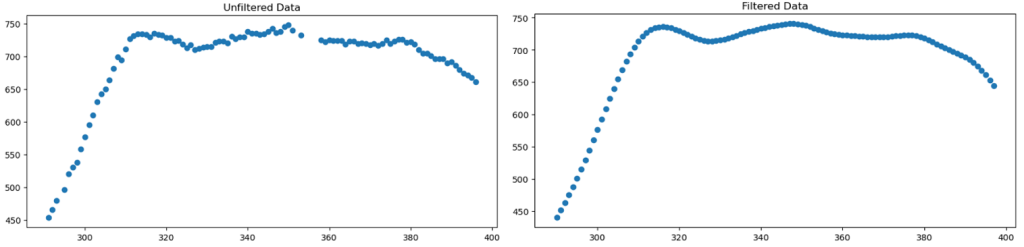
When we attempted to apply a fourth-degree Butterworth filter, we found it was smoothing out these crucial high-frequency components, effectively erasing the most important part of our signal – the rapid acceleration phase of the swing. Even reducing to a second-degree filter didn’t solve the problem; we were still losing vital information about the swing’s peak velocity phase.
The Swingathon and Model Refinement
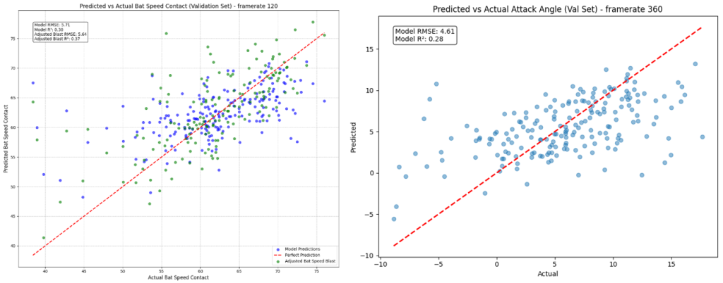
In December 2024, we recognized that our model, while performing well for bat speeds between 50-75 mph, needed improvement outside this range. This led to an intensive data collection effort we dubbed “The Swingathon” – a 15-hour session capturing 900 swings with various bat types and swing characteristics.
These tee-based swings required us to modify our point of contact detection algorithm. We developed a method that analyzed the ball’s pixel position changes (delta) frame by frame. One significant advantage of this approach was its independence from swing direction – the algorithm worked equally well for both right and left-handed hitters without requiring video flipping. A stationary ball on the tee would have a delta of zero, making the initial state easy to identify.
When the bat made contact, it would cause a significant change in the ball’s delta, giving us a rough window of frames where contact likely occurred.
However, identifying the exact point of contact required more precision. We used a two-step process: first, the change in delta helped us identify a narrow range of potential contact frames. Then, within this range, we performed a frame-by-frame analysis of the distance between the ball and the bat’s sweet spot to pinpoint the exact frame of contact. This hybrid approach combined the efficiency of delta-based detection with the precision of spatial analysis.
Keypoint Confidences
A pose estimation model generates two types of confidence scores: object detection confidence (how certain it is about identifying the object and its bounding box) and keypoint confidence (how certain it is about the specific keypoint locations). Initially, we were filtering our predictions based solely on object detection confidence, requiring a threshold of 0.85 or higher. This approach, while seemingly conservative, was actually causing us to discard potentially valuable data.
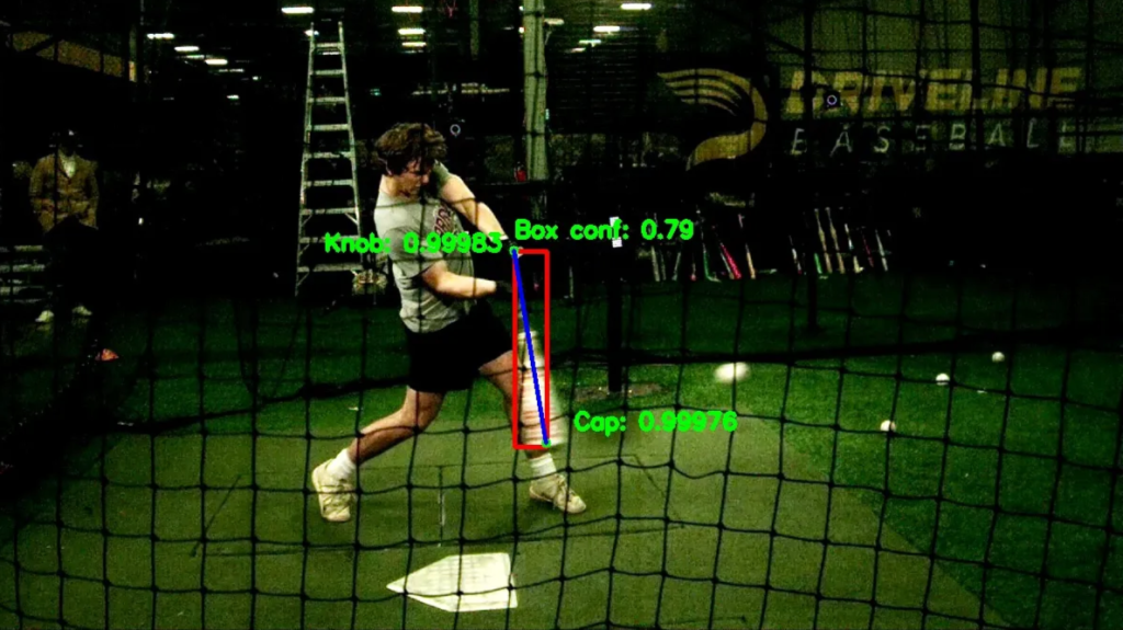
Yet another breakthrough came when we began investigating the relationship between these two confidence types. Our analysis revealed something surprising: even in frames where object detection confidence was low (often due to motion blur), the model was frequently making accurate keypoint predictions. This insight led us to launch a comprehensive investigation into keypoint confidence reliability.
We manually annotated 3,200 images, focusing particularly on cases where our original pipeline had struggled (object detection < 0.8). These were frames that our previous approach would have discarded and interpolated. For each image, we compared the ground truth pixel coordinates with our model’s predictions, analyzing both the miss distances and the model’s reported confidence in each prediction.
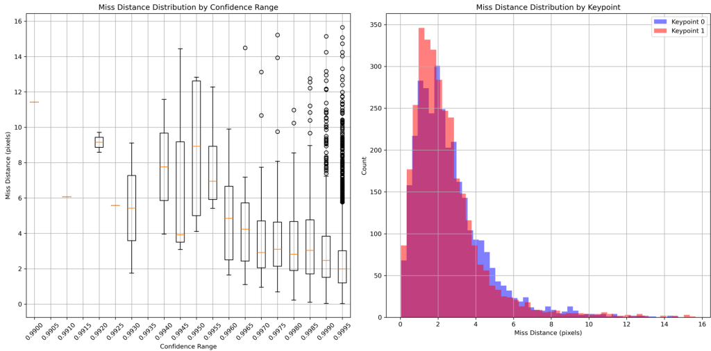
The results were revealing. Our model’s keypoint predictions were remarkably accurate, with maximum miss distances of only 14-15 pixels even in challenging cases. After filtering obvious outliers (confidence < 0.99), the statistical analysis showed impressive precision:
Knob Keypoint Statistics
| Statistic | Confidence | Miss Distance (pixels) |
|---|---|---|
| Count | 3236 | 3236 |
| Mean | 0.999590 | 2.6262 |
| Standard Deviation | 0.000465 | 1.9098 |
| Minimum | 0.992733 | 0.0413 |
| 25th Percentile | 0.999581 | 1.3077 |
| Median (50th %) | 0.999720 | 2.1717 |
| 75th Percentile | 0.999807 | 3.3687 |
| Maximum | 0.999948 | 14.7283 |
Cap Keypoint Statistics
| Statistic | Confidence | Miss Distance (pixels) |
|---|---|---|
| Count | 3193 | 3193 |
| Mean | 0.999610 | 2.4354 |
| Standard Deviation | 0.000531 | 1.9019 |
| Minimum | 0.990198 | 0.0345 |
| 25th Percentile | 0.999588 | 1.2188 |
| Median (50th %) | 0.999742 | 2.0070 |
| 75th Percentile | 0.999820 | 3.0375 |
| Maximum | 0.999949 | 15.6513 |
These findings revolutionized our approach to swing analysis:
- Independent Keypoint Evaluation
- Previously, if either the cap or knob confidence was low, we would discard the entire frame. Our statistical analysis showed that often one keypoint would maintain high confidence even when the other struggled. By evaluating keypoints independently, we could now keep the high-confidence keypoint and only interpolate the other. This immediately reduced our data loss by approximately 50% in problematic frames.
- Selective Interpolation
- Before this analysis, we were interpolating an average of 10 frames per video due to poor object detection confidence. This not only created potential inaccuracies but also required significant computational overhead. With our new keypoint-based approach, we virtually eliminated the need for interpolation. When interpolation is needed, it’s now targeted to specific keypoints rather than entire frames, preserving more of the original data.
- Salvaging “Poor” Bounding Box Predictions
- Perhaps most significantly, we discovered that a poor bounding box confidence didn’t necessarily indicate poor keypoint detection. In frames with motion blur, the model might struggle to define the exact boundaries of the bat (leading to low box confidence) while still accurately identifying the cap and knob positions. This insight allowed us to keep many frames we previously would have discarded, particularly during the crucial high-speed portions of swings.
These improvements dramatically reduced the need for additional model training. Previously, we might have concluded that more annotation was needed to improve performance in motion-blurred frames. Instead, by better utilizing our existing predictions, we’ve created a more robust system while actually reducing computational overhead.
Real-Time Processing Pipeline
A critical requirement of our system was the ability to generate bat speed predictions quickly enough to be useful for our same day motion capture reports. To achieve this, we developed an automated processing pipeline that begins the moment a swing is recorded.
We implemented a watchdog script that continuously monitors our camera system for new videos. As soon as our side-view camera captures a swing, the script automatically identifies the new file and immediately begins processing. This automation eliminates any manual steps between video capture and analysis, allowing us to generate bat speed predictions within 10 seconds of the swing.
This rapid processing capability was essential for efficiently pairing our predictions with the corresponding mocap data and maintaining an organized database of swing analyses. The quick turnaround time ensures that coaches and players can access swing data immediately following their motion capture session in the Launchpad.
Engineering Precision through LOESS Refinement
Every measurement system requires calibration, and our bat speed prediction model was no exception. As we analyzed our results, we discovered systematic variations between our predictions and actual measurements – variations that followed subtle but consistent patterns across different speeds and angles.
To address these patterns, we implemented a LOESS (Locally Estimated Scatterplot Smoothing) calibration system. This statistical approach allowed us to map the relationship between our initial predictions and actual measurements with remarkable precision. By applying this calibration curve to our predictions, we could automatically adjust for any systematic variations in our model’s output.
The development of this calibration system presented its own engineering challenges. We needed to determine the optimal allocation of our dataset between training, validation, and testing phases. Through careful analysis, we discovered that we could use our real-time predictions as a natural test set, allowing us to dedicate more data to developing our calibration curve without compromising our model’s base performance.
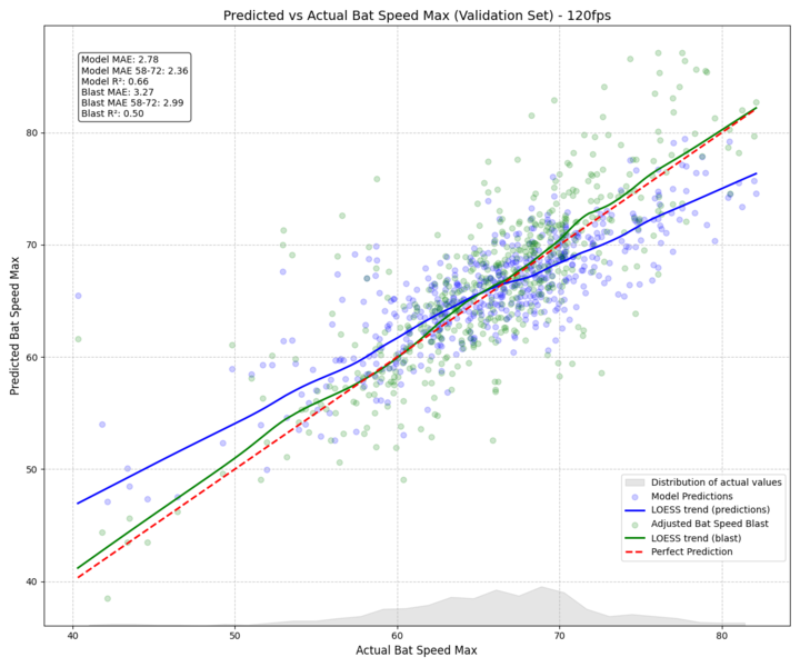
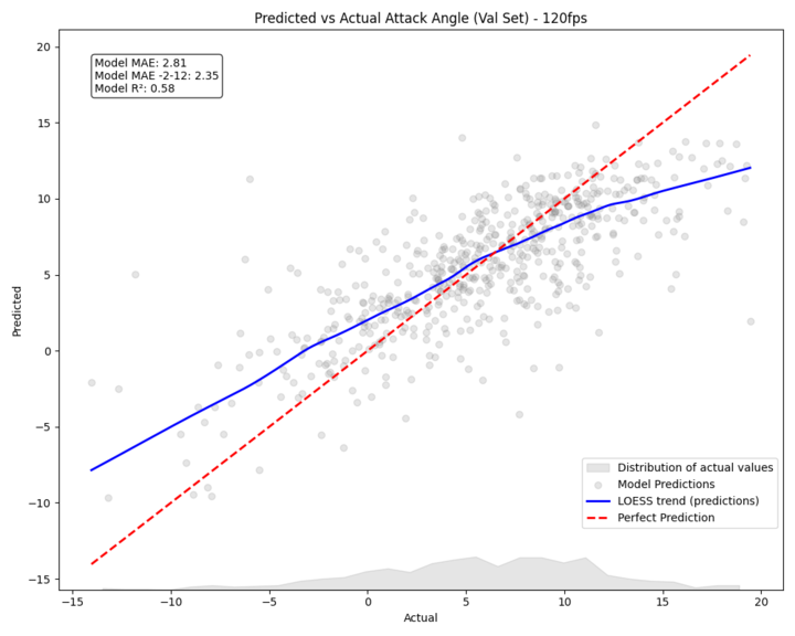
The results exceeded our expectations. Our calibrated system now produces highly accurate measurements across the full range of bat speeds and attack angles. For example, if our system initially predicts a bat speed of 70 mph, our calibration adjusts it to 73.09 mph, bringing it in line with our motion capture measurements. Similarly, attack angle predictions are refined with impressive precision – a raw prediction of 8 degrees is adjusted to 8.99 degrees, matching our ground truth data.
Adjusted Bat Speeds (mph)
50.00 -> 46.64
55.00 -> 51.68
60.00 -> 56.65
65.00 -> 64.32
70.00 -> 73.09
75.00 -> 79.03
80.00 -> 84.95
Adjusted Attack Angles (degrees)
-8.00 -> -18.59
-4.00 -> -10.93
0.00 -> -3.65
4.00 -> 2.66
8.00 -> 8.99
12.00 -> 16.95
16.00 -> 27.32
As with any precision measurement system, we’re continuing to refine our calibration through extensive real-world testing. Over the coming months, we’ll be collecting additional validation data to ensure our calibration remains accurate across all possible scenarios.
Conclusion: Beyond Bat Speed
Our journey from initial concept to working system has been one of continuous problem-solving and innovation. What began as a simple bat-tracking project evolved into a sophisticated system that bridges the gap between computer vision and biomechanics. The challenges we encountered – from depth perception to signal processing – pushed us to develop novel solutions that may have applications beyond baseball.
The success of our scaling factor approach demonstrates that sometimes the simplest solutions are the most elegant. By using the bat itself as a measuring stick, we solved a complex 3D reconstruction problem without the need for multiple cameras or complex depth estimation algorithms. This principle of finding simple, robust solutions to complex problems guided our entire development process.
Looking ahead, we see numerous possibilities for expanding this system. The ability to accurately track bat movement from a single camera view opens doors for applications ranging from amateur player development to professional game analysis. We could potentially extend this methodology to other sports equipment or movement analysis where traditional motion capture systems are impractical.
Most importantly, this project has shown that with careful consideration of the underlying physics and biomechanics, computer vision can provide reliable quantitative measurements from simple video input. As we continue to refine our system, we’re excited about the potential to make sophisticated swing analysis more accessible to players and coaches at all levels of the game.
Editor’s Note: Driveline Baseball filed for intellectual property protection under the US Patent and Trademark Office on this technology in 2024. Reference # US 63/634,678.